Full notes

Table of contents

• L1 Systems of linear equations, Gaussian elimination
  • Key Concepts:
  • Formulas and Definitions:
  • Examples:
  • Important Theorems and Proofs:
• L2 Vector and matrix equations
  • Key Concepts:
  • Formulas and Definitions:
  • Examples:
  • Important Theorems and Proofs:
• L3 Solution sets, linear independence
  • Key Concepts:
  • Formulas and Definitions:
  • Examples:
  • Important Theorems and Proofs:
• L4 Linear transformations, matrix algebra
  • Key Concepts:
  • Formulas and Definitions:
  • Examples:
  • Important Theorems and Proofs:
• L5 Perspective projections, inverse of matrices
  • Key Concepts:
  • Formulas and Definitions:
  • Examples:
  • Important Theorems and Proofs:
• L6 Determinants
  • Key Concepts:
  • Formulas and Definitions:
  • Examples:
  • Important Theorems and Proofs:
  • Calculating determinants
  • Calculating the inverse of a matrix
• L7 Vector spaces
  • Key Concepts:
  • Formulas and Definitions:
  • Examples:
  • Important Theorems and Proofs:
• L8 More about vector spaces
  • Key Concepts:
  • Formulas and Definitions:
  • Examples:
  • Important Theorems and Proofs:
• L9 Eigenvalues and Eigenvectors
  • Key Concepts:
  • Formulas and Definitions:
  • Examples:
  • Important Theorems and Proofs:
  • Concrete examples
• L10 Diagonalization
  • Key Concepts:
  • Formulas and Definitions:
  • Examples:
  • Important Theorems and Proofs:
  • Applications:
• L11 Orthogonality and symmetric matrices
  • Key Concepts:
  • Formulas and Definitions:
  • Examples:
  • Important Theorems and Proofs:
  • Concrete examples
    • Testing for Orthogonality:
    • Testing for Orthonormality:

L1 Systems of linear equations, Gaussian elimination

BCS1410-1 Lecture 1

Key Concepts:

• Systems of Linear Equations: Solutions of sets of equations that work for all equations within the set, representing lines in ${\mathbb{R}}^2$.
• Unique Solution: If the system of linear equations (SLE) has a unique solution, it can be efficiently found through Gaussian elimination.
• Row Echelon Form (REF): A form of a matrix where each leading entry is to the right of the leading entry in the previous row.
• Gaussian Elimination: A method for solving SLEs, involving three types of row operations: replacement, scaling, and interchange.

Formulas and Definitions:

• Augmented Matrix: Combines the coefficients of the variables and the constants from the equations of an SLE into a single matrix.
• Row Equivalence: Two matrices are row equivalent if one can be obtained from the other by a series of row operations.
• Consistent SLE: An SLE that has at least one solution.
• Inconsistent SLE: An SLE that has no solution, typically indicated by a row where all the variable coefficients are 0, but the constant is non-zero.

Examples:

• SLE with No Solutions: Exhibits a row like $[00|10]$ after Gaussian elimination.
• SLE with Infinitely Many Solutions: Appears when the system describes lines that overlap, indicating an infinite number of intersection points.
• Parametric Form: A way to express the solution set when there are infinitely many solutions.

Important Theorems and Proofs:

• Pivot Positions: In REF, a pivot is the first non-zero entry in a row, and all entries above and below in its column are zero.
• Reduced Row Echelon Form (RREF): A further refinement of REF, where each leading entry is the only non-zero entry in its column, making it unique for a matrix.

---

L2 Vector and matrix equations

BCS1410-2 Lecture 2

Key Concepts:

• Matrix Equations: Viewed as a column perspective to an SLE, especially useful in applications like machine learning where columns represent features.
• Feature Vectors: Data points in feature space, such as height and weight from a number of animals, which can be vectors in ${\mathbb{R}}^n$.
• Linear Combination: The vector $\sum c_i{\mathbf{v}}_i$ is called a linear combination of vectors ${\mathbf{v}}_1,{\mathbf{v}}_2,...,{\mathbf{v}}_p$ with weights $c_1,c_2,...,c_p$.

Formulas and Definitions:

• Scaling and Addition: Fundamental operations with vectors; for example, scaling a vector by 2 or adding two vectors together.
• Vector Equation: An equation like $a_1{\mathbf{v}}_1+a_2{\mathbf{v}}_2=\mathbf{b}$, which is equivalent to an SLE.

Examples:

• Column View of an SLE: Investigating whether a vector $\mathbf{b}$ can be written as a linear combination of the columns of a matrix $A$.
• Parametric Vector Form: Expresses the solution set to an SLE with many solutions in ${\mathbb{R}}^n$; for example, $3\mathbf{u}+\mathbf{w}$ where $\mathbf{w}$ is any scalar multiple of $\mathbf{u}$.

Important Theorems and Proofs:

• Matrix Equation: Given by $A\mathbf{x}=\mathbf{b}$ and has the same solution set as the corresponding vector equation and SLE.
• Consistency: An SLE is consistent if and only if the vector $\mathbf{b}$ is in the column space of $A$; this is equivalent to saying that there exist weights $c_i$ such that $A\mathbf{x}=\mathbf{b}$.

---

L3 Solution sets, linear independence

BCS1410-3 Lecture 3

Key Concepts:

• Homogeneous SLE: An SLE of the form $Ax=0$ is always consistent because it has at least the trivial solution (all zeros).
• Non-homogeneous SLE: An SLE of the form $Ax=b$, where $b\ne 0$. The solution set is the sum of a particular solution of the non-homogeneous SLE and the solution set of the corresponding homogeneous SLE.
• Linear Independence: A set of vectors $\{v_1,v_2,...,v_n\}$ is linearly independent if the only solution to $c_1{v}_1+c_2{v}_2+...+c_n{v}_n=0$ is $c_1=c_2=...=c_n=0$.

Formulas and Definitions:

• Trivial Solution: In the context of a homogeneous SLE, it is the solution where all variables are set to zero.
• Linear Combination: Form $v=c_1{v}_1+c_2{v}_2+...+c_n{v}_n$ represents a linear combination of vectors with coefficients $c_1,c_2,...,c_n$.

Examples:

• Testing for Linear Independence: To test a set of vectors for linear independence, transform the matrix formed by these vectors to REF and look for pivot positions in every column.
• Single Vector Linear Independence: Any non-zero vector is linearly independent by itself.
• Zero Vector: A set containing the zero vector is always linearly dependent.

Important Theorems and Proofs:

• Set of Solutions for Non-homogeneous SLE: The solution set can be written as the set of all vectors of the form $v_p+v_h$, where $v_p$ is a particular solution to the non-homogeneous SLE and $v_h$ is any solution to the corresponding homogeneous SLE.
• Linear Dependence with Zero Vector: If the set includes the zero vector, it is linearly dependent because a non-trivial combination can give zero by using zero coefficients for other vectors and a non-zero coefficient for the zero vector.

---

L4 Linear transformations, matrix algebra

BCS1410-4 Lecture 4

Key Concepts:

• Matrix Algebra and Transformations: Focus on linear transformations and their representation through matrices.
• Linear Transformations: Functions that map vectors from one vector space to another, preserving vector addition and scalar multiplication.
• Matrix Vector Product: A transformation of a vector $\mathbf{x}$ by a matrix $A$ resulting in a vector $\mathbf{b}$, denoted as $A\mathbf{x}=\mathbf{b}$.
• Examples of Linear Transformations: Including rotation, reflection, and projection, which are all linear transformations.

Formulas and Definitions:

• Linear Transformation: A transformation $T$ is linear if it satisfies $T(\mathbf{x}+\mathbf{y})=T(\mathbf{x})+T(\mathbf{y})$ and $T(c\mathbf{x})=cT(\mathbf{x})$ for all vectors $\mathbf{x},\mathbf{y}$ in its domain and scalar $c$.
• Matrix Representation of Linear Transformations: The standard matrix for a linear transformation $T$ from ${\mathbb{R}}^n$ to ${\mathbb{R}}^m$ is the matrix $A$ such that $T(\mathbf{x})=A\mathbf{x}$ for all $\mathbf{x}$ in ${\mathbb{R}}^n$.

Examples:

• Rotation about the Origin: Represented by a matrix $A$ that rotates vectors by a specified angle.
• Reflection: Represented by a matrix that reflects vectors across a specified axis or line.
• Projection onto an Axis: Represented by a matrix that projects vectors onto a specified axis.

Important Theorems and Proofs:

• Injectivity and Surjectivity of Linear Transformations: A linear transformation is injective (one-to-one) if and only if it maps distinct vectors to distinct vectors, and surjective (onto) if every vector in the codomain is the image of at least one vector from the domain.
• Matrix Algebra Properties: Including the properties of matrix addition, scalar multiplication, and the special cases of the transpose and symmetric matrices.

Transpose matrices

Symmetry for Square Matrices

• Definition: A square matrix $A$ is symmetric if $A=A^T$.
• Implication: The matrix is equal to its transpose.

Transpose of a Transpose

• Property: $(A^T{)}^T=A$
• Implication: Applying the transpose operation twice returns the original matrix.

Transpose of a Sum

• Property: $(A+B{)}^T=A^T+B^T$
• Implication: The transpose of a sum is the sum of the transposes.

Transpose of a Product

• Property: $(AB{)}^T=B^T{A}^T$
• Implication: When matrices are multiplied, the order of multiplication is reversed in the transpose.

Transpose of a Scalar Multiplication

• Property: $(cA{)}^T=c{A}^T$ where $c$ is a scalar.
• Implication: Scalar multiplication is distributive over the transpose operation.

Rank

• Property: $rank(A)=rank(A^T)$
• Implication: The rank of a matrix is unchanged by transposition.

Determinant

• Property: $det(A)=det(A^T)$ for square matrices.
• Implication: The determinant of a matrix is the same as its transpose.

Inverse

• Property: If $A$ is invertible, then $(A^T{)}^{-1}=(A^{-1}{)}^T$.
• Implication: The inverse of the transpose is the transpose of the inverse.

Eigenvalues

• Property: The eigenvalues of $A$ are the same as the eigenvalues of $A^T$.
• Implication: Transposition does not affect the eigenvalues of a matrix.

Orthogonal Matrices

• Property: A square matrix $A$ is orthogonal if $A^{T}A=A{A}^T=I$, where $I$ is the identity matrix. For such matrices, $A^T$ is also the inverse of $A$: $A^T=A^{-1}$.
• Implication: Orthogonal matrices preserve lengths and angles.

---

L5 Perspective projections, inverse of matrices

BCS1410-5 Lecture 5

Key Concepts:

• Inverse of a Matrix: The concept of an inverse matrix is crucial for solving systems of linear equations, among other applications.
• Homogeneous Coordinates: Used in computer graphics to represent three-dimensional objects on a two-dimensional screen.
• Elementary Matrices: Result from performing a single elementary row operation on an identity matrix. They are crucial for finding the inverse of a matrix.

Formulas and Definitions:

• Elementary Row Operations: Include replacement (adding multiples of one row to another), scaling (multiplying a row by a non-zero scalar), and interchange (swapping two rows).
• Invertible Matrix (Nonsingular Matrix): A square matrix $A$ is invertible if there exists a matrix $A^{-1}$ such that $A{A}^{-1}=A^{-1}A=I$, where $I$ is the identity matrix.

Examples:

• Finding the Inverse of a Matrix: Involves applying a series of elementary row operations to transform the matrix into the identity matrix, while performing the same operations on the identity matrix to obtain the inverse.
• Application in Computer Graphics: Homogeneous coordinates are employed to easily perform linear transformations, like rotation and translation, on points and vectors in a 3D space projected onto a 2D plane.

Important Theorems and Proofs:

• Criteria for Invertibility: ==A square matrix $A$ is invertible if it is row equivalent to the identity matrix and it has a pivot position in every row (and column).==
• Uniqueness of the Inverse: The inverse of a matrix, if it exists, is unique. This uniqueness is fundamental for the stability and predictability of many mathematical and computational procedures.
• Algorithm for Finding $A^{-1}$: The process to find $A^{-1}$ involves Gaussian elimination or applying a series of elementary row operations to reduce $A$ to $I$, simultaneously transforming $I$ into $A^{-1}$.

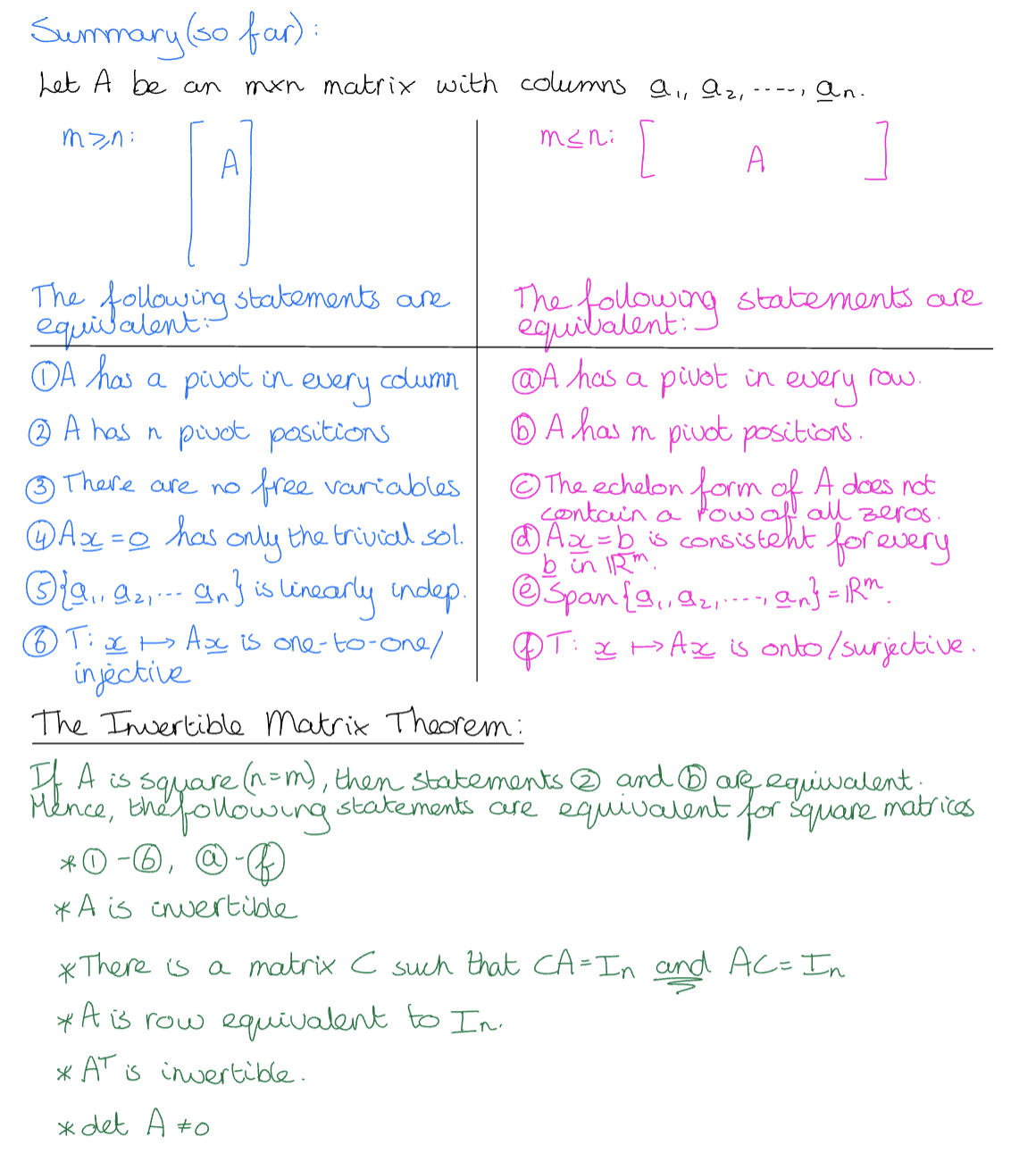
Invertible Matrix Theorem

The Invertible Matrix Theorem is a central result in linear algebra that provides a list of equivalent statements, which, if true for a square matrix $A$, imply that $A$ is invertible (and conversely, if any of these statements is false, then $A$ is not invertible). This theorem links various concepts in linear algebra, showing their interdependence. Here are the key points of the theorem, summarized in bullet points:

[!note ] Square Matrix $A$ is Invertible This is the foundational statement that the rest of the conditions either affirm or deny.

• Determinant: $det(A)\ne 0$. A matrix is invertible if and only if its determinant is non-zero.
• Matrix Rank: The rank of $A$ equals its number of columns (or rows), indicating full rank.
• Unique Solutions: The equation $A\mathbf{x}=\mathbf{b}$ has a unique solution for every vector $\mathbf{b}$ in ${\mathbb{R}}^n$.
• Null Space: The null space of $A$ contains only the zero vector, i.e., $N(A)=\{0\}$.
• Column Space: The columns of $A$ span ${\mathbb{R}}^n$, making them linearly independent.
• Row Equivalence: The matrix $A$ is row equivalent to the identity matrix $I_n$.
• Inverse Existence: There exists an $n\times n$ matrix $A^{-1}$ such that $A{A}^{-1}=A^{-1}A=I_n$.
• Eigenvalues: $A$ has no zero eigenvalues. Any zero eigenvalue would imply a determinant of zero, contradicting invertibility.
• Transpose Invertibility: The transpose $A^T$ is invertible.
• Subspaces: The column space and row space of $A$ are equal to ${\mathbb{R}}^n$.
• Linear Transformations: The linear transformation mapping $\mathbf{x}$ to $A\mathbf{x}$ is both one-to-one and onto, covering the entire space without overlap or omission.
• Product of Invertible Matrices: If $A$ can be expressed as a product of elementary matrices, then it is invertible, as elementary matrices are invertible.

This theorem elegantly ties together different properties and concepts regarding square matrices, showing how they provide various perspectives on the idea of invertibility. The equivalence of these conditions means that verifying any one of them for a particular matrix guarantees that all the other conditions hold true as well, offering multiple pathways to determine or utilize the invertibility of a matrix in problem-solving.

---

L6 Determinants

BCS1410-6 Lecture 6

Key Concepts:

• Inverse Matrix and Cryptography: Explores the application of inverse matrices in cryptography, such as the Hill cipher algorithm.
• Determinant of a Matrix: A scalar associated with a square matrix, indicating how a transformation changes area or volume.
• Cofactor Expansion: Method for calculating the determinant of a matrix by expanding along a row or column.

Formulas and Definitions:

• Determinant Notation: Denoted as $\text{det}(A)$ or $|A|$, measures the scaling factor of the transformation represented by matrix $A$.
• Homogeneous Coordinates: Used in graphical applications to manage dimensions and perspective transformations efficiently.
• Elementary Matrices: Arise from performing elementary row operations on the identity matrix, instrumental in deriving the inverse of a matrix.

Examples:

• Determinant and Area Scaling: Demonstrates how the determinant reflects the scaling of areas or volumes, such as stretching or compressing.
• Invertibility and Determinants: A matrix is invertible if and only if its determinant is non-zero.

Calculating determinants

To calculate the determinant of a matrix, different formulas and methods are used depending on the size of the matrix. Here are some common formulas for calculating determinants:

• 2x2 Matrix: For a matrix $A=\left(\begin{array}{cc}a& b\\ c& d\end{array}\right)$, the determinant is calculated as: $\text{det}(A)=ad-bc$
• 3x3 Matrix: For a matrix $A=\left(\begin{array}{ccc}a& b& c\\ d& e& f\\ g& h& i\end{array}\right)$, the determinant can be calculated using the rule of Sarrus: $\text{det}(A)=aei+bfg+cdh-ceg-bdi-afh$
• nxn Matrix (General Case): For larger matrices, the determinant can be calculated using cofactor expansion. For any row $i$ or column $j$, the determinant of matrix $A$ is: $\text{det}(A)={\sum }_{j=1}^n(-1{)}^{i+j}{a}_{ij}\text{det}(A_{ij})$ where $a_{ij}$ is the element in the $i^{th}$ row and $j^{th}$ column, and $A_{ij}$ is the matrix obtained by removing the $i^{th}$ row and $j^{th}$ column from $A$ (this is called the minor of $A$ at $a_{ij}$).

The sign $(-1{)}^{i+j}$ is positive if the sum of the row and column indices is even, and negative if the sum is odd, ensuring the correct sign based on the position of the element in the matrix.

• Special Cases and Properties:
  • Triangular Matrices (both upper and lower): The determinant is the product of the diagonal elements.
  • Determinant of the Identity Matrix: The determinant of the identity matrix of any size is 1.
  • Determinant of a Product: The determinant of a product of matrices equals the product of their determinants: $\text{det}(AB)=\text{det}(A)\cdot \text{det}(B)$.
  • Inverse and Determinant: A square matrix $A$ is invertible if and only if $\text{det}(A)\ne 0$. If $A$ is invertible, then $\text{det}(A^{-1})=1/\text{det}(A)$.

Calculating the inverse of a matrix

To calculate the inverse of a matrix, it’s crucial to understand that not all matrices have inverses. A square matrix $A$ has an inverse, denoted as $A^{-1}$, if there exists a matrix that, when multiplied by $A$, results in the identity matrix $I$. Here’s how to calculate the inverse of a matrix, with examples:

• Formula to Calculate Inverse of a 2x2 Matrix: For a 2x2 matrix $A=\left(\begin{array}{cc}a& b\\ c& d\end{array}\right)$, the inverse is given by: $A^{-1}=\frac{1}{\text{det}(A)}\left(\begin{array}{cc}d& -b\\ -c& a\end{array}\right)=\frac{1}{ad-bc}\left(\begin{array}{cc}d& -b\\ -c& a\end{array}\right)$ where $\text{det}(A)=ad-bc$ is the determinant of $A$. The matrix $A$ is invertible if and only if $\text{det}(A)\ne 0$.

• Example for 2x2 Matrix: Let $A=\left(\begin{array}{cc}4& 7\\ 2& 6\end{array}\right)$. The determinant $\text{det}(A)=(4)(6)-(7)(2)=24-14=10$. Thus, the inverse of $A$ is: $A^{-1}=\frac{1}{10}\left(\begin{array}{cc}6& -7\\ -2& 4\end{array}\right)=\left(\begin{array}{cc}0.6& -0.7\\ -0.2& 0.4\end{array}\right)$

• Formula for nxn Matrix Using Elementary Row Operations: For larger matrices, the inverse can be found by augmenting the matrix $A$ with the identity matrix $I$ of the same size, and then performing elementary row operations to transform $A$ into $I$. The operations that transform $A$ into $I$ will transform $I$ into $A^{-1}$ on the augmented side.

1. Write the augmented matrix $(A|I)$.
2. Use row operations to transform $A$ into the identity matrix.
3. The matrix that appears where $I$ was is $A^{-1}$.

• Example for 3x3 Matrix: Consider $A=\left(\begin{array}{ccc}1& 2& 3\\ 0& 1& 4\\ 5& 6& 0\end{array}\right)$. To find $A^{-1}$, augment $A$ with the identity matrix and apply row operations to transform $A$ into $I$. This process is more complex and requires multiple steps, so we won’t solve it fully here. However, the methodology follows the described procedure.
• Important Notes:
  • Existence of Inverse: A square matrix $A$ is invertible if and only if $\text{det}(A)\ne 0$.

---

L7 Vector spaces

BCS1410-7 Lecture 7

Key Concepts:

• Vector Spaces: Fundamental concept in linear algebra, encompassing sets of vectors in any dimension, including functions, polynomials, and more.
• Subspaces: A subset of a vector space that is itself a vector space under the same addition and scalar multiplication operations.

Formulas and Definitions:

• Definition of a Vector Space: A set $V$ of vectors is a vector space if it is closed under vector addition and scalar multiplication. For any vectors $\mathbf{u},\mathbf{v}\in V$ and scalar $c$, the set is closed under addition $(\mathbf{u}+\mathbf{v}\in V)$ and scalar multiplication $(c\mathbf{v}\in V)$.
• Subspaces: A subset $W$ of a vector space $V$ is a subspace of $V$ if $W$ itself satisfies the vector space properties (closure under addition and scalar multiplication, contains the zero vector).

Examples:

• Real Numbers as a Vector Space: The set of all real numbers $\mathbb{R}$ is a basic example of a vector space.
• Polynomials of Degree at Most $n$: The set of all polynomials with degree at most $n$, denoted $P_n$, is a vector space.
• Subspaces in ${\mathbb{R}}^n$: For any matrix $A$, the set of all vectors that are solutions to the homogeneous system $A\mathbf{x}=0$ forms a subspace of ${\mathbb{R}}^n$.

Important Theorems and Proofs:

• Criteria for Subspaces: A subset $W$ of $V$ is a subspace if it contains the zero vector and is closed under vector addition and scalar multiplication.
• Subspace Example with Polynomials: The set of polynomials of a certain degree forms a subspace, as it includes the zero polynomial and is closed under addition and scalar multiplication.

---

L8 More about vector spaces

BCS1410-11 Lecture 11

Key Concepts:

• Basis and Dimension: Fundamental concepts for understanding vector spaces, including how to construct a vector space and the minimum number of vectors needed for its basis.
• Nul(A), Col(A), and Row(A): Essential subspaces associated with any matrix $A$, representing the null space, column space, and row space, respectively.

Formulas and Definitions:

• Basis of a Vector Space: A set of vectors in a vector space $V$ that is linearly independent and spans $V$. The number of vectors in a basis is the dimension of $V$, denoted as $\text{dim}(V)$.
• Null Space (Nul A): The set of all vectors $\mathbf{x}$ such that $A\mathbf{x}=0$. A basis for $\text{Nul}(A)$ can be found by solving $A\mathbf{x}=0$ and expressing the solution set in vector form.
• Column Space (Col A): The set of all linear combinations of the columns of $A$. A basis for $\text{Col}(A)$ can be found from the pivot columns of $A$ in its reduced echelon form.
• Row Space (Row A): The set of all linear combinations of the rows of $A$. A basis for $\text{Row}(A)$ corresponds to the non-zero rows in the reduced echelon form of $A$.

Examples:

• Basis for ${\mathbb{R}}^3$: The standard basis is $\{\left(\begin{array}{c}1\\ 0\\ 0\end{array}\right),\left(\begin{array}{c}0\\ 1\\ 0\end{array}\right),\left(\begin{array}{c}0\\ 0\\ 1\end{array}\right)\}$.
• Basis for a Polynomial Space $P_n$: The set of polynomials of degree at most $n$ has a basis of $\{1,x,x^2,\dots ,x^n\}$.
• Subspaces: For any matrix $A$, $\text{Nul}(A)$, $\text{Col}(A)$, and $\text{Row}(A)$ are subspaces of appropriate ${\mathbb{R}}^n$ or ${\mathbb{R}}^m$ spaces, with dimensions giving key insights into the properties of $A$.

Important Theorems and Proofs:

• Invertible Matrix Theorem: Connects the concept of an invertible matrix with properties like being row equivalent to the identity matrix, having a non-zero determinant, and the absence of free variables for uniqueness of solutions to systems of linear equations.
• Subspace Criterion: A subset $W$ of a vector space $V$ is a subspace if and only if it is non-empty, closed under vector addition and scalar multiplication, and contains the zero vector.

---

L9 Eigenvalues and Eigenvectors

BCS1410-11 Lecture 11

Key Concepts:

• Eigenvalues and Eigenvectors: Fundamental concepts in linear algebra that describe vectors that only change by a scalar factor when a linear transformation is applied.
• Characteristic Polynomial: A polynomial that is instrumental in finding the eigenvalues of a matrix.

Formulas and Definitions:

• Eigenvalue and Eigenvector Definition: For a square matrix $A$, a scalar $\lambda$ is an eigenvalue if there exists a non-zero vector $\mathbf{v}$ such that $A\mathbf{v}=\lambda \mathbf{v}$. The vector $\mathbf{v}$ is called an eigenvector corresponding to $\lambda$.
• Characteristic Polynomial: Given by $\text{det}(A-\lambda I)=0$, where $I$ is the identity matrix of the same size as $A$. Solving this equation for $\lambda$ gives the eigenvalues of $A$.
• Eigenspace: The set of all eigenvectors corresponding to a particular eigenvalue $\lambda$, along with the zero vector, forms a subspace related to $A$ called the eigenspace of $\lambda$.

Examples:

• Finding Eigenvalues: For matrix $A$, solve $\text{det}(A-\lambda I)=0$ to find eigenvalues $\lambda$.
• Finding Eigenvectors: Once eigenvalues $\lambda$ are known, solve $(A-\lambda I)\mathbf{v}=0$ to find the corresponding eigenvectors $\mathbf{v}$.

Important Theorems and Proofs:

• Invertibility and Eigenvalues: A matrix $A$ is invertible if and only if $0$ is not an eigenvalue of $A$.
• Trace and Determinant: The trace of $A$, denoted $\text{tr}(A)$, is the sum of eigenvalues of $A$, and the determinant of $A$, $\text{det}(A)$, is the product of its eigenvalues.

Concrete examples

To illustrate the process of finding eigenvalues and eigenvectors, let’s go through a detailed example with a 2x2 matrix. This process involves two main steps: finding the eigenvalues and then finding the eigenvectors corresponding to those eigenvalues.

Step 1: Finding Eigenvalues

Consider the matrix $A=\left(\begin{array}{cc}4& 1\\ 2& 3\end{array}\right)$.

1. Determine the characteristic equation by calculating the determinant of $A-\lambda I$, where $I$ is the identity matrix, and $\lambda$ represents the eigenvalues of $A$.

   $\text{det}(A-\lambda I)=\text{det}\left(\left(\begin{array}{cc}4& 1\\ 2& 3\end{array}\right)-\left(\begin{array}{cc}\lambda & 0\\ 0& \lambda \end{array}\right)\right)=\text{det}\left(\begin{array}{cc}4-\lambda & 1\\ 2& 3-\lambda \end{array}\right)$

   $=(4-\lambda )(3-\lambda )-(2)(1)={\lambda }^2-7\lambda +10=0$

2. Solve the characteristic equation for $\lambda$.

   ${\lambda }^2-7\lambda +10=0$ The solutions to this quadratic equation are the eigenvalues. In this case, ${\lambda }_1=2$ and ${\lambda }_2=5$.

Step 2: Finding Eigenvectors

Once the eigenvalues are determined, we find the eigenvectors by solving $(A-\lambda I)\mathbf{v}=0$ for each eigenvalue.

• For ${\lambda }_1=2$:

  1. Substitute ${\lambda }_1$ into the equation and solve for $\mathbf{v}$.

  $\left(\begin{array}{cc}4-2& 1\\ 2& 3-2\end{array}\right)\left(\begin{array}{c}x\\ y\end{array}\right)=\left(\begin{array}{c}0\\ 0\end{array}\right)$

  $\left(\begin{array}{cc}2& 1\\ 2& 1\end{array}\right)\left(\begin{array}{c}x\\ y\end{array}\right)=\left(\begin{array}{c}0\\ 0\end{array}\right)$

  1. Solving this system, we find that $x=-y$. We can choose $y=1$, so an eigenvector corresponding to ${\lambda }_1=2$ is ${\mathbf{v}}_1=\left(\begin{array}{c}-1\\ 1\end{array}\right)$.

• For ${\lambda }_2=5$:

  1. Substitute ${\lambda }_2$ into the equation and solve for $\mathbf{v}$. $\left(\begin{array}{cc}4-5& 1\\ 2& 3-5\end{array}\right)\left(\begin{array}{c}x\\ y\end{array}\right)=\left(\begin{array}{c}0\\ 0\end{array}\right)$ $\left(\begin{array}{cc}-1& 1\\ 2& -2\end{array}\right)\left(\begin{array}{c}x\\ y\end{array}\right)=\left(\begin{array}{c}0\\ 0\end{array}\right)$
  2. Solving this system, we find that $x=y$. Choosing $x=1$, an eigenvector corresponding to ${\lambda }_2=5$ is ${\mathbf{v}}_2=\left(\begin{array}{c}1\\ 1\end{array}\right)$.

---

L10 Diagonalization

BCS1410-11 Lecture 11

Key Concepts:

• Diagonalization: A matrix $A$ is diagonalizable if it is similar to a diagonal matrix, meaning there exists an invertible matrix $P$ such that $P^{-1}AP$ is a diagonal matrix.
• Eigenvalues and Eigenvectors: Essential for the process of diagonalization, where eigenvalues populate the diagonal of the diagonal matrix, and eigenvectors form the columns of matrix $P$.

Formulas and Definitions:

• Diagonal Matrix: A square matrix in which the entries outside the main diagonal are all zero. The main diagonal can contain any scalar, including the eigenvalues of $A$.
• Similar Matrices: Two matrices $A$ and $B$ are similar if $B=P^{-1}AP$, where $P$ is an invertible matrix.
• Theorem on Eigenvalues: Similar matrices have the same eigenvalues.

Examples:

• Diagonalization Process:
  1. Find Eigenvalues: Solve $\text{det}(A-\lambda I)=0$ for $\lambda$ to find the eigenvalues of $A$.
  2. Find Eigenvectors: For each eigenvalue $\lambda$, solve $(A-\lambda I)\mathbf{x}=0$ to find the corresponding eigenvectors.
  3. Form Matrix $P$: Assemble a matrix $P$ using the eigenvectors as columns.
  4. Compute $P^{-1}AP$: The result is a diagonal matrix $D$ with eigenvalues on the diagonal.
• Example with Specific Matrix:
  • Given $A=\left(\begin{array}{cc}2& 1\\ 1& 2\end{array}\right)$, find eigenvalues ${\lambda }_1=3$ and ${\lambda }_2=1$, and corresponding eigenvectors ${\mathbf{v}}_1=\left(\begin{array}{c}1\\ 1\end{array}\right)$ and ${\mathbf{v}}_2=\left(\begin{array}{c}-1\\ 1\end{array}\right)$. Matrix $P$ is $\left(\begin{array}{cc}1& -1\\ 1& 1\end{array}\right)$, and $P^{-1}AP=\left(\begin{array}{cc}3& 0\\ 0& 1\end{array}\right)$.

Important Theorems and Proofs:

• Diagonalizability Criteria: A matrix $A$ is diagonalizable if it has $n$ linearly independent eigenvectors. If $A$ has $n$ distinct eigenvalues, it is automatically diagonalizable.

Applications:

• Solving Differential Equations: Diagonalization simplifies the process of solving systems of linear differential equations.
• Efficient Computation: Powers of matrices can be easily computed when the matrix is diagonalizable.

---

L11 Orthogonality and symmetric matrices

BCS1410-11 Lecture 11

Key Concepts:

• Symmetric Matrices: A central topic of the lecture, where the matrix is equal to its transpose, i.e., $A=A^T$.
• Inner Dot Product: The dot product is an algebraic operation that takes two equal-length sequences of numbers and returns a single number. It is expressed as $\vec{u}\cdot \vec{v}$.
• Length (Norm) of a Vector: Given by $||\vec{v}||=\sqrt{\vec{v}\cdot \vec{v}}$, it represents the magnitude of the vector.
• Unit Vector: A vector with a length of 1, calculated as $\vec{u}=\frac{\vec{v}}{||\vec{v}||}$.
• Distance Between Two Vectors: The Euclidean distance given by $\text{dist}(\vec{u},\vec{v})=||\vec{u}-\vec{v}||$.
• Orthogonal Vectors: Two vectors are orthogonal if their dot product is zero, i.e., $\vec{a}\cdot \vec{b}=0$.
• Null Space of a Matrix (Nul A): All vectors $\vec{x}$ such that $A\vec{x}=\vec{0}$. Every vector in Nul A is orthogonal to every vector in Row A.

Formulas and Definitions:

• Orthogonal Set: A set of vectors is orthogonal if the dot product between each pair of distinct vectors is zero.
• Orthonormal Set: An orthogonal set of vectors where each vector has a length of 1.
• Orthogonal Matrix: A square matrix A is orthogonal if $A^{T}A=I$, meaning its transpose is also its inverse.
• Orthogonal Projection: Projecting vector y onto the subspace spanned by an orthogonal basis.
• Orthogonal Basis: A basis of a subspace where all the basis vectors are orthogonal to each other.

Examples:

• Orthogonality in Applications: Important for feature detection in signal processing and statistics.
• Testing for Orthogonality: To check if a set $\{e_n\}$ is orthogonal, form matrix A from the vectors and calculate $A^{T}A$. If $A^{T}A$ is diagonal, $\{e_n\}$ is orthogonal. If $A^{T}A$ is the identity matrix, $\{e_n\}$ is orthonormal.
• Diagonalization: A matrix A is orthogonally diagonalizable if it is symmetric, meaning $A=PD{P}^T$ where D is diagonal and P is orthogonal.

Important Theorems and Proofs:

• Eigenvectors from different eigenvalues are orthogonal in the context of symmetric matrices.
• The dimensionality relationship: $\text{dim}(W)+\text{dim}(W^{\perp })=n$, where $W^{\perp }$ is the orthogonal complement of W in ${\mathbb{R}}^n$.

Concrete examples

Testing for Orthogonality:

1. Example 1:

   • Consider two vectors ${\mathbf{v}}_1=\left(\begin{array}{c}1\\ -2\\ 3\end{array}\right)$ and ${\mathbf{v}}_2=\left(\begin{array}{c}2\\ 1\\ 4\end{array}\right)$.
   • To test for orthogonality, compute their dot product: ${\mathbf{v}}_1\cdot {\mathbf{v}}_2=1(2)+(-2)(1)+3(4)=2-2+12=12$.
   • Since the dot product is not zero, the vectors are not orthogonal.

2. Example 2:

   • Given two vectors $\mathbf{u}=\left(\begin{array}{c}3\\ -1\\ 0\end{array}\right)$ and $\mathbf{v}=\left(\begin{array}{c}2\\ 6\\ -3\end{array}\right)$.
   • Compute their dot product: $\mathbf{u}\cdot \mathbf{v}=3(2)+(-1)(6)+0(-3)=6-6+0=0$.
   • Since the dot product is zero, the vectors are orthogonal.

Testing for Orthonormality:

1. Example 1:

   • Consider a set of three vectors in ${\mathbb{R}}^3$: ${\mathbf{v}}_1=\left(\begin{array}{c}1\\ 0\\ 0\end{array}\right)$, ${\mathbf{v}}_2=\left(\begin{array}{c}0\\ 1\\ 0\end{array}\right)$, and ${\mathbf{v}}_3=\left(\begin{array}{c}0\\ 0\\ 1\end{array}\right)$.
   • To test for orthonormality, compute the dot products between each pair of vectors. They should all equal 0 except when the vectors are the same, where it should equal 1.
   • For example, ${\mathbf{v}}_1\cdot {\mathbf{v}}_2=1(0)+0(1)+0(0)=0$, ${\mathbf{v}}_1\cdot {\mathbf{v}}_1=1(1)+0(0)+0(0)=1$.
   • Repeat this process for all pairs of vectors to confirm orthonormality.

2. Example 2:

   • Given an orthonormal basis: $\{{\mathbf{u}}_1,{\mathbf{u}}_2,{\mathbf{u}}_3\}$, where each vector has a length of 1 and they are mutually orthogonal.
   • To test orthonormality, compute the dot products as above. Each dot product should be 0 except for dot products of a vector with itself, which should be 1.